Others
Others
Documentation for the other usable functions equipped in SeaGap.
Site information file
SeaGap often requires site location; thus, it is convenient to instantly obtain site information. read_info(site,filename) is a simple function to obtain the basic site information from a file filename.
If you prepare a following file named "site_info.txt" with the site information (1: Site name, 2: Longitude [deg], 3: Latitude [deg], 4: Water depth [m], 5: Total number of transponders):
$ cat site_info.txt
G01 144.953750000 38.697035000 5490.2 4
G02 144.047013333 40.737111667 4672.5 4
G03 143.967245000 40.126088333 4218.4 4
G04 143.897145000 39.566171667 4586.5 6
G05 143.316761667 39.325555000 2084.8 4
G06 143.849871667 39.302598333 4770.4 4
G07 143.940026667 38.942755000 5550.4 3
G08 143.647465000 38.721148333 3473.1 4
G09 143.791663333 38.480898333 5646.5 4
G10 143.482881667 38.301606667 3270.8 6
G11 143.801736667 38.266500000 5548.5 4
G12 143.531633333 38.020813333 4370.4 3
G13 143.198573333 37.932891667 2480.5 4
G14 142.774661667 37.891595000 1312.0 4
G15 143.520901667 37.677226667 5263.9 6
G16 143.048235000 37.333650000 4406.7 4
G17 142.715440000 36.899033333 4232.4 4
G18 141.982523333 36.615520000 2490.6 4
G19 142.670803333 36.496250000 5724.8 6
G20 142.082610000 36.157530000 2742.7 4
you can obtain the values at a certain site site as following:
julia> lon, lat, wd, numk = SeaGap.read_info("G20","site_info.txt")
(142.08261, 36.15753, 2742.7, 4)
julia> lat
36.15753
Date & Time processing
date -> cal
date2cal() transforms "date" into "cumulative days in year".
year, cal = SeaGap.date2cal("2015-10-01")
(2015, 274)
If you use this function as date2cal.(), you can handle a vector input and transform multiple values.
Moreover, date2cal_txt(fn0,fn) reads a text file (fn0 is the input file name) with dates in the first row and writes a text file (fn is the output file name) after transformation.
If preparing the following text file:
$ cat test01.txt
2015-10-10T12:00:00 100
2015-12-10T12:00:00 200
2016-02-10T12:00:00 300
and performing the following:
SeaGap.date2cal_txt("test01.txt","test1.txt")you can obtain the following output file:
$ cat test1.txt
2015 283 100
2015 344 200
2016 041 300
date -> year
date2year() transforms "date" into "year".
year, cal = SeaGap.date2year("2015-10-01")
2015.7506849315068
If you use this function as date2year.(), you can handle a vector input and transform multiple values.
Moreover, date2year_txt(fn0,fn) reads a text file (fn0 is the input file name) with dates in the first row and writes a text file (fn is the output file name) after transformation.
If preparing the above text file (test01.txt) and performing the following:
SeaGap.date2year_txt("test01.txt","test1.txt")you can obtain the following output file:
$ cat test1.txt
2015.775342465754 100
2015.942465753425 200
2016.112021857924 300
date -> sec
date2sec(t,t0) transforms "date" into "cumulative seconds from the reference date". The reference date t0 is set to 2000-01-01T12:00:00 as the defalt value.
sec = SeaGap.date2sec("2015-10-01T12:34:56")
4.96974896e8
sec = SeaGap.date2sec("2015-10-01T12:34:56",t0="2015-01-01T12:00:00")
2.3589296e7
If you use this function as date2sec.(), you can handle a vector input and transform multiple values.
Moreover, date2sec_txt(fn0,fn,t0) reads a text file (fn0 is the input file name) with dates in the first row and writes a text file (fn is the output file name) after transformation.
If preparing the above text file (test01.txt) and performing the following:
SeaGap.date2sec_txt("test01.txt","test1.txt")you can obtain the following output file:
$ cat test1.txt
497750400.000000 100
503020800.000000 200
508377600.000000 300
sec -> date
sec2date(t,t0) and sec2date_txt(fn0,fn,t0) work as reverse functions of date2sec(t,t0) and date2sec_txt(fn0,fn,t0), respectively.
sec -> year
sec2year(t,t0) and sec2year_txt(fn0,fn,t0) convert "cumulative seconds from the reference date" into "year". The reference date t0 is set to 2000-01-01T12:00:00 as the defalt value.
SeaGap.sec2year(4.969728e8)
2015.7506849315068
If preparing the following text file (test02.txt)
497750400.000000 100
503020800.000000 200
508377600.000000 300
and performing the following:
SeaGap.sec2year_txt("test02.txt","test2.txt")you can obtain the following output file:
$ cat test2.txt
2015.775342465754 100
2015.942465753425 200
2016.112021857924 300
Coordinate transformation
SeaGap perform coordinate transformation between geographic coordinate and a projection coordinate by "mapproject" module in GMT. The projection system is Transverse Mercator (-Jt).
Longitude, Latitude -> XY
ll2xy(lon,lat,lon0,lat0) transforms the geographic coordinate (lon and lat) into the projection coordinate with the projection center of (lon0, lat0)
x, y = SeaGap.ll2xy(139.01,37.99,139,38)
(878.4438672769625, -1109.9166351306528)
If you'd like to transform multiple values, you can use ll2xy_vec(lon,lat,lon0,lat0). In this case, lon and lat are vectors with the same dimensions.
If you'd like to transform multiple values via a text file, you can use ll2xy_txt(fn0,fn,ks,lon0,lat0). fn0 is the input file written in the geographic coordinate, and fn is the output file written in the projected coordinate. ks is an identifer for the longitude row. If the longitude and latitude are shown in the rows 1 and 2, you set ks=1; if the longitude and latitude are shown in the rows 3 and 4, you set ks=3.
$ head gps.jllhpr
500663320.00 142.077767915 36.182468927 27.875250 -4.5784 -1.4752 0.2540
500663320.50 142.077771912 36.182447992 27.644200 -4.4348 -1.0296 -0.5176
500663321.00 142.077775355 36.182427602 27.533200 -4.2144 -0.8856 -1.0988
500663321.50 142.077778539 36.182407813 27.577200 -3.9376 -1.0300 -1.4052
500663322.00 142.077782024 36.182388370 27.688650 -3.6868 -1.2688 -1.4408
500663322.50 142.077786287 36.182368782 27.709300 -3.5284 -1.3532 -1.2196
500663323.00 142.077791670 36.182348941 27.534550 -3.4464 -1.1888 -0.7060
500663323.50 142.077797880 36.182329011 27.240900 -3.3472 -0.8852 0.0952
500663324.00 142.077804425 36.182309198 26.938300 -3.1948 -0.6000 1.0656
500663324.50 142.077810868 36.182289402 26.737900 -3.0584 -0.3556 1.9636
The above file can be transformed as following:
SeaGap.ll2xy_txt("gps.jllhhpr","hoge.txt",2,142.082610,36.157530)$ head hoge.txt
500663320.00 -435.572296 2767.287953 27.875250 -4.5784 -1.4752 0.2540
500663320.50 -435.212860 2764.964938 27.644200 -4.4348 -1.0296 -0.5176
500663321.00 -434.903255 2762.702399 27.533200 -4.2144 -0.8856 -1.0988
500663321.50 -434.616946 2760.506550 27.577200 -3.9376 -1.0300 -1.4052
500663322.00 -434.303558 2758.349093 27.688650 -3.6868 -1.2688 -1.4408
500663322.50 -433.920185 2756.175543 27.709300 -3.5284 -1.3532 -1.2196
500663323.00 -433.436064 2753.973914 27.534550 -3.4464 -1.1888 -0.7060
500663323.50 -432.877549 2751.762406 27.240900 -3.3472 -0.8852 0.0952
500663324.00 -432.288897 2749.563879 26.938300 -3.1948 -0.6000 1.0656
500663324.50 -431.709421 2747.367239 26.737900 -3.0584 -0.3556 1.9636
XY -> Longitude, Latitude
In SeaGap, the reverse functions for ll2xy(),ll2xy_vec(), and ll2xy_txt() are provided as xy2ll(), xy2ll_vec(), and xy2ll_txt(), respectively.
Sorting
As for the tuple type, Julia's sort function works as similar with Unix's sort command (if you sort for one certain column, the other columns are also sorted following the certain column's order). However, as for the array or matrix types, Julia's sort function works differently (only the selected column is sorted). Then, SeaGap provides new sort functions unixsort(x,k) and unixsort2(x,k1,k2) which also works for the array and matrix types as similar with Unix's sort command but only works for numerical values.x is array or matrix, and k is number of the column to be sorted. As for unixsort2(x,k1,k2), k1 is the primary column to be sorted and k2 is the secondary column to be sorted.
a = hcat(round.(rand(10)),rand(10,3))
10×4 Matrix{Float64}:
 1.0  0.825768   0.43119    0.915429
 0.0  0.136709   0.520284   0.171813
 1.0  0.579633   0.911675   0.364961
 1.0  0.0203354  0.616683   0.515084
 1.0  0.605135   0.56349    0.808185
 0.0  0.448877   0.710546   0.130922
 1.0  0.426983   0.43761    0.369329
 1.0  0.280084   0.641669   0.163034
 1.0  0.199115   0.896918   0.224157
 0.0  0.402337   0.0203177  0.600175
a_new = SeaGap.unixsort(a,2)
10×4 Matrix{Float64}:
1.0 0.0203354 0.616683 0.515084
0.0 0.136709 0.520284 0.171813
1.0 0.199115 0.896918 0.224157
1.0 0.280084 0.641669 0.163034
0.0 0.402337 0.0203177 0.600175
1.0 0.426983 0.43761 0.369329
0.0 0.448877 0.710546 0.130922
1.0 0.579633 0.911675 0.364961
1.0 0.605135 0.56349 0.808185
1.0 0.825768 0.43119 0.915429a_new = SeaGap.unixsort2(a,1,3)
10×4 Matrix{Float64}:
0.0 0.402337 0.0203177 0.600175
0.0 0.136709 0.520284 0.171813
0.0 0.448877 0.710546 0.130922
1.0 0.825768 0.43119 0.915429
1.0 0.426983 0.43761 0.369329
1.0 0.605135 0.56349 0.808185
1.0 0.0203354 0.616683 0.515084
1.0 0.280084 0.641669 0.163034
1.0 0.199115 0.896918 0.224157
1.0 0.579633 0.911675 0.364961Running filter
SeaGap provides simple running (moving) filters: runmed(x,k) and runave(x,k) which are a running median filter and a running average filter, respectively. Both functions smooth the input numerical vector x by k length of a running window.
Preparing input data with 1-dimension array:
using Distributions
t = collect(range(1,10,10))
a = collect(range(1,10,10))+rand(Cauchy(),10)
10-element Vector{Float64}:
  0.9713071965257543
  3.4732347973689537
  2.3512497164125667
  4.076701783766254
 15.169399082762245
 -7.814884216883062
  7.515355534078403
  7.350965798485638
  9.776065411160495
  9.200257419697813
Performing the running median and average filters with 3 length running window:
a_med = SeaGap.runmed(a,3)
a_ave = SeaGap.runave(a,3)
Plotting the results:
using Plots
plt = plot(t,a,label="Raw")
plot!(plt,t,a_med,label="Median")
plot!(plt,t,a_ave,label="Average")
savefig(plt,"filter_test.png")
Simple inversion
simple_inversion(d,H) is a function performing a simple least mean squares method. d is a data vector, and H is a kernel matrix. The obervation equation is given using a solution vector a as following:
a is simply obtained as:
Then, we can calculate a synthetic data vector as and a residual vector as . Moreover, we can calculate covariance matrix for the estimated paramters as:
with
Note that and is the length of the data and model vectors,respectively. Then, we can obtain a standard deviation vector . simple_inversion(d,H) returns the , , , and .
dcal, dres, a, e = SeaGap.simple_inversion(d,H)Line fit
linefit(x,y,w0;alpha,newX) is a function of a least squares method for simple line fitting: . x and y are vectors with the same length, and they must be occupied. wo is a weight vector, and you can optionally use it. alpha is a real value with range between 0 and 1, and alpha*100 indicates the percentage for confidentional intervals; linefit() provides the upper and lower confidentional intervals for the fitting line. The default alpha is set to be 0.95, which means 95% CI. newX is an optional vector; if you assign newX, the predicted values, the upper and lower confidentional intervals following newX are provided: .
If you have following vectors:
julia> t
10-element Vector{Float64}:
  1.0
  2.0
  3.0
  4.0
  5.0
  6.0
  7.0
  8.0
  9.0
 10.0
julia> a
10-element Vector{Float64}:
0.9713071965257543
3.4732347973689537
2.3512497164125667
4.076701783766254
15.169399082762245
-7.814884216883062
7.515355534078403
7.350965798485638
9.776065411160495
9.200257419697813julia> t_new = collect(range(1,10,20))
20-element Vector{Float64}:
1.0
1.4736842105263157
1.9473684210526316
2.4210526315789473
2.8947368421052633
3.3684210526315788
3.8421052631578947
4.315789473684211
4.7894736842105265
5.2631578947368425
5.7368421052631575
6.2105263157894735
6.684210526315789
7.157894736842105
7.631578947368421
8.105263157894736
8.578947368421053
9.052631578947368
9.526315789473685
10.0you can perform the line fitting without wights as following:
lf = SeaGap.linefit(t,a,newX=t_new)In the above case, lf contains the whole estimation results. lf.coef has the estimated coefficients for A and B
A, B = lf.coef
2-element Vector{Float64}:
 0.8566110967793089
 0.7909734828287631
lf.coefstd has standard deviations for the estimated coefficients of A and B
A_std, B_std = lf.coefstd
2-element Vector{Float64}:
 4.1435872512068945
 0.6677995520930635
lf.pred and lf.misfit are prediction and misfit values:
hcat(t,lf.pred,lf.misfit)
10×3 Matrix{Float64}:
  1.0  1.64758   -0.676277
  2.0  2.43856    1.03468
  3.0  3.22953   -0.878282
  4.0  4.02051    0.0561968
  5.0  4.81148   10.3579
  6.0  5.60245  -13.4173
  7.0  6.39343    1.12193
  8.0  7.1844     0.166567
  9.0  7.97537    1.80069
10.0 8.76635 0.433911lf.pred_new, lf.pred_upper, and lf.pred_lower are prediction, the upper and lower confidential intervals following newX, respectively:
hcat(t_new,lf.pred_new,lf.pred_upper,lf.pred_lower)
20×4 Matrix{Float64}:
  1.0      1.64758   9.86866  -6.57349
  1.47368  2.02226   9.63858  -5.59406
  1.94737  2.39693   9.43218  -4.63833
  2.42105  2.7716    9.25585  -3.71265
  2.89474  3.14627   9.1179   -2.82535
  3.36842  3.52094   9.02906  -1.98717
  3.84211  3.89561   9.00272  -1.2115
  4.31579  4.27029   9.05463  -0.514063
  4.78947  4.64496   9.20145   0.0884669
  5.26316  5.01963   9.45781   0.581452
  5.73684  5.3943    9.83248   0.956124
  6.21053  5.76897  10.3255    1.21248
  6.68421  6.14364  10.928     1.3593
  7.15789  6.51832  11.6254    1.41121
  7.63158  6.89299  12.4011    1.38487
  8.10526  7.26766  13.2393    1.29603
  8.57895  7.64233  14.1266    1.15808
  9.05263  8.017    15.0523    0.981748
  9.52632  8.39167  16.008     0.775353
 10.0      8.76635  16.9874    0.54527
Plotting them as:
using Plots
plt = scatter(t,a,label="Raw")
plot!(plt,t,lf.pred,label="Prediction")
plot!(plt,t_new,lf.pred_upper,label="Upper CI")
plot!(plt,t_new,lf.pred_lower,label="Lower CI")
savefig(plt,"line_fit-test.png")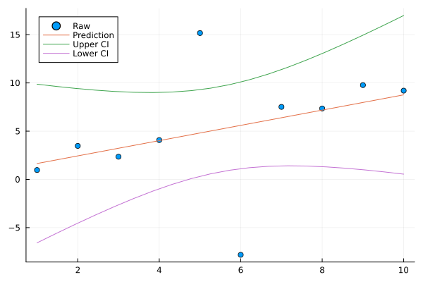
CC BY-SA 4.0 Fumiaki Tomita. Last modified: July 03, 2024.
Website built with Franklin.jl and the Julia programming language.