Forward calculation

Here, synthetic calculation of travel-times is performed to practice handling SeaGap.

You first prepare an underwater sound profile ("ss_prof.inp": See Dataformat).

0.00 1526.998
5.00 1529.598
10.00 1529.594
15.00 1529.637
20.00 1529.684
25.00 1529.748
30.00 1529.343
35.00 1528.586
40.00 1527.722
45.00 1525.194

SeaGap prepares the read function for "ss_prof.inp" read_prof(fn,TR_DEPTH). fn is the file name (such as fn="ss_prof.inp"). TR_DEPTH is the depth of the sea-surface transponder from the sea-surface. Although TR_DEPTH changes depending on attitudes of the sea-surface platform, it is enough to roughly provide its average value. This value is used for identifying which sound speed layer of "ss_prof.inp" the transducer exists.

TR_DEPTH = 3.0
z, v, nz_st, numz = SeaGap.read_prof("ss_prof.inp",TR_DEPTH)

Performing the above (TR_DEPTH is set as 3.0), you obtain z (depth value vector), v (velocity value vector), nz_st (number of layer that the transducer exists), and numz (total number of layers).

Next, you should obtain a local Earth radius. Using localradius(lat), you can obtain a Gaussian mean radius and a local mean radius (Chadwell & Sweeney, 2010). They do not show significant difference for calculating a travel-time; therefore, SeaGap generally uses the Gaussian mean radius.

For tha case lat=38.0,

Rg, Rl = SeaGap.localradius(38.0)
(6.372923169901545e6, 6.372909276228537e6)

Rg is the Gaussian mean radius, and Rl is the local mean radius.

Then, you can calculate one-way exact travel-times (see Methodology) by xyz2tt(px,py,pz,xd,yd,zd,z,v,nz_st,numz,Rg,TR_DEPTH) where px, py, and pz are position of a seafloor transponder, and xd, yd, and zd are position of a sea-surface transducer. Unit of these positions is meter.

px = 1500.0; py = 0.0; pz = -3000.0
xd = 100.0; yd = -100.0; zd = -1.5 
tc, Nint, vert = SeaGap.xyz2tt(px,py,pz,xd,yd,zd,z,v,nz_st,numz,Rg,TR_DEPTH)
(2.220777604567047, 4, 0.9057269733438277)

tc is the one-way travel-time, Nint is the total number of iterations in the shooting method, and vert is the normalizing factor corresponding to $\frac{1}{M}$ shown in Methodlogy.

If you'd like to calculate the approximate travel-time (see Methodology), you have to run ttcorrection(px,py,pz,tr_height,z,v,nz_st,numz,TR_DEPTH,lat) in advance. Then, you can calculate the approximate travel-time by xyz2tt_rapid()

tr_height = -1.0
Tv0, Vd, Vr, cc, rms = SeaGap.ttcorrection(px,py,pz,tr_height,z,v,nz_st,numz,TR_DEPTH,lat)

You have to provide tr_height which is the mean height of the sea-surface transponder; if you have time-series of the sea-surface transponder height as zd, tr_height=Statistics.mean(zd). But, note that rough value is acceptable for tr_height within a few meters.

Tv0, Vd, Vr, and cc is correction paramters for performing xyz2tt_rapid().rms is RMS between the exact and the approximate travel-times when optimizing.

Then, xyz2tt_rapid() can be performed as following:

tc_r, to_r, vert_r = SeaGap.xyz2tt_rapid(px,py,pz,xd,yd,zd,Rg,Tv0,Vd,Vr,tr_height,cc)
(2.2207776042517358, 2.2207913746628574, 0.9057269733438277)

tc_r is the approximate travel-time,to_r is the simple spherical travel-time ($T_{\rm Sphere}$), and vert_r is the same with vert.

Moreover, SeaGap equips another function to calculate the approximate travel-time: xyz2ttg_rapid().

tc_g, vert_g, hh_x, hh_y = SeaGap.xyz2ttg_rapid(px,py,pz,xd,yd,zd,Rg,Tv0,Vd,Vr,tr_height,cc)
(2.2207776042517358, 0.9057269733438277, 0.4669001167250292, 0.03335000833750208)

tc_g and vert_g are same with tc_r and vert_r, respectively. hh_x and hh_y are coefficients for expressing a deep gradient (See Methodology).

If you'd like to obtain travel-times from various sea-surface points, you can do it like:

xdv = Float64[]; ydv = Float64[]; zdv = Float64[]; tcv = Float64[]
  yd = 0.
  for xd in 0:100:2000
    # --- Set z-value randomly from -5 to 0
    zd = rand()*-5.0
    # --- Calculate TT
    tc, Nint, vert = xyz2tt(px,py,pz,xd,yd,zd,z,v,nz_st,numz,Rg,TR_DEPTH)
    push!(xdv,xd); push!(ydv,yd); push!(zdv,zd); push!(tcv,tc)
  end

Then, you can obtain as:

hcat(xdv,ydv,zdv,tcv)
21×4 Matrix{Float64}:
    0.0  0.0  -0.961723  2.24927
  100.0  0.0  -2.29837   2.21929
  200.0  0.0  -1.91723   2.19199
  300.0  0.0  -3.31861   2.16533
  400.0  0.0  -2.87221   2.14159
  500.0  0.0  -2.65163   2.11956
  600.0  0.0  -4.79642   2.09794
  700.0  0.0  -3.84929   2.08025
  800.0  0.0  -0.492697  2.06614
  900.0  0.0  -1.43069   2.05133
 1000.0  0.0  -1.98022   2.03887
 1100.0  0.0  -4.57954   2.02721
 1200.0  0.0  -0.366569  2.02222
 1300.0  0.0  -4.26667   2.01407
 1400.0  0.0  -1.53643   2.01252
 1500.0  0.0  -0.325024  2.01221
 1600.0  0.0  -4.35567   2.01065
 1700.0  0.0  -3.82967   2.01435
 1800.0  0.0  -3.66194   2.02004
 1900.0  0.0  -0.855999  2.02966
 2000.0  0.0  -1.55564   2.03915

You can test the above calculation by forward_test(lat,TR_DEPTH,pos,fn="ss_prof.inp") with pos is a position vector of a seafloor trannsponder pos = [px,py,pz].

xdv, ydv, zdv, tcv = SeaGap.forward_test(lat,TR_DEPTH,[px,py,pz],fn="ss_prof.inp")

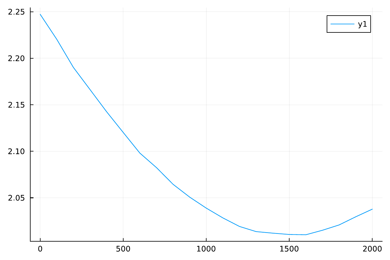
using Plots # Drawing figure
plot(xdv,tcv)

You can check how the travel-times vary depending on the horizontal distance by the plotted figure. The horizontal axis indicates the horizontal distance in meter, and the vertical axis indicates the calculated travel-times in sec.