Tutorials
MCMC static array positioning
- Make initial value file
- Make initial value file generated from the least square method
- Run MCMC processing
- Output text files
- Visualization
- Posterior PDF and RMS variation through the MCMC iteration
- Parameter variation through the MCMC iteration
- Correlation among the unknown parameters
- Histogram for each unknown parameter
- Histograms and heatmaps for multiple parameters
- Spatial variation of travel-time residuals (shallow gardient)
- Temporal variation of the travel-time residuals
The static array positioning methods considering a sound speed gradient through a MCMC technique in Tomita & Kido, 2022 was implemented as static_array_mcmcgrad.jl, and its slightly updated version was also implemented as Tomita & Kido, 2024. However, these methods are outdated from SeaGap v1.1.0. The highly improved MCMC method (under review) is implemented as static_array_mcmcgradv(). The SeaGap developer strongly recommend to use static_array_mcmcgradv.jl.
Make initial value file
Firstly, we have to prepare an initial value file (named "initial.inp" by default) which lists initial values of the unknown parameters for performing static_array_mcmcgradv().
The dataformat of "initial.inp" is (Columns 1: Initial value, 2: Step width, 3: Parameter name). The step width is used as perturbation (Metropolis method) when new parameter candidates are produced during the MCMC chain. This should be appropriately given to effectively perform a MCMC sampling.
The type of unknown parameters to be placed on each line of this file is fixed and cannot be changed.
Lines 1-3: Array displacements for EW, NS, UD [m]
Lines 4-5: Shallow gradients for EW, NS [sec/km]
Lines 6-7: Gradient depths for EW, NS [km]
Line 8: Scaling factor for the observational error
Line 9: Scaling factor for temporal S-NTD roughness
Line 10: Scaling factor for temporal shallow gradient roughness
Line 11: Scaling factor for temporal gradient depth roughness
Lines 7-11: Long-term NTD modeled by 4th polynomial function (degree: 0-4)
Lines 12-(12+NPB1): Coefficients for the 3d B-spline bases of L-NTD
Lines (13+NPB1)-: Coefficients for the 3d B-spline bases of S-NTD
This file can be produced by make_initial_gradv(NPB1, NPB2; fn, fno) function using the results of static array positioning method static_array_s(). In static_array_mcmcgradv(), NTD is decomposed into L-NTD and S-NTD. They are expressed by the 3d B-spline functions, and their total numbers of spline bases are NPB1 and NPB2, respectively. Tomita (under review) fixed NPB1 as 5 and NPB2 as the number determined by BIC in static_array() and static_array_AICBIC().
Make initial value file generated from the least square method
static_array_s() estimates a static array position, L-NTD, S-NTD, and the shallow gradients (temporally-fixed) by Gauss-Newton method. This method is introduced in Tomita (under review). To solve these parameters, we need to constrain L2-norm of S-NTD using a hyper-parameter alpha.
lat=36.15753; TR_DEPTH=[4.0]; NPB1=5; NPB2=73; alpha = 0.0
SeaGap.static_array_s(lat,TR_DEPTH,alpha,NPB1,NPB2,fno1="solve.out")
SeaGap.plot_ntd_s(fno="ntd_s.png")
You can check the travel time residuals in this modelling by plot_ntd_s().
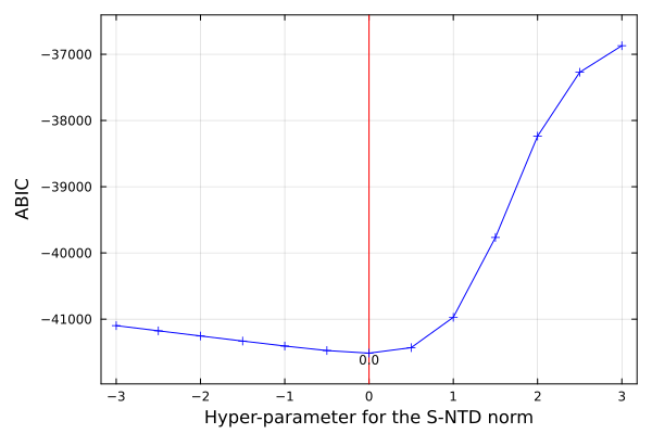
fno1 includeis the estimates, and this file is used for making the initial value. alpha is typically zero, but the optimal value of alpha can be evaluated by ABIC. The optimization using the ABIC value is performed by static_array_s_ABIC()
r1=-3.0; r2=3.0; r3=0.5
SeaGap.static_array_s_ABIC(r1,r2,r3,lat,TR_DEPTH,NPB1,NPB2)
SeaGap.plot_ABIC(show=true)r1, r2, and r3 are lower limit, upper limit, and interval of the hyper-parameter range, respectively.
Using solve.out obtained from static_array_s(), you can obtain the initial value file for MCMC.
SeaGap.make_initial_gradv(NPB1,NPB2)$ head -n 20 initial.inp
0.025410462308784486 0.0003285916454800491 EW_disp.
-0.01569704833998688 0.00032709528235116216 NS_disp.
-0.03417871494024675 0.00119971349382272 UD_disp.
-8.37248428698407e-5 2.0e-6 S-Grad_EW
8.89971826238189e-5 2.0e-6 S-Grad_NS
0.0 0.01 G-Depth_EW
0.0 0.01 G-Depth_NS
-4.0 0.005 HP_error
-4.5 0.005 HP_S-NTD
-4.5 0.005 HP_S-Grad
-1.0 0.005 HP_G-Depth
0.001885751243719274 2.0e-6 L-NTD_1
0.0019299017374440242 2.0e-6 L-NTD_2
0.0017720436581544553 2.0e-6 L-NTD_3
0.0024791239571273424 2.0e-6 L-NTD_4
0.005824457411845061 2.0e-6 L-NTD_5
0.0 2.0e-6 S-NTD_1
0.0 2.0e-6 S-NTD_2
0.0 2.0e-6 S-NTD_3
0.0 2.0e-6 S-NTD_4
Run MCMC processing
Before you run static_array_mcmcgradv(), you have to set number of threads for the thread parallelization in your terminal as:
$ export JULIA_NUM_THREADS=4
or you have to run Julia as:
$ julia -t 4
This value is determined depending on your machine ability.
Then, after setting the above thread number and preparing the above input files, you can perform static_array_mcmcgrad(lat,TR_DEPTH,NPB; NSB,nloop,nburn,ndelay,NA,lscale,daave,daind,tscale,fn1,fn2,fn3,fn4,fn5,fno0,fno1,fno2,fno3,fno4,fno5,fno6,fno7) function as following:
lat=36.15753; TR_DEPTH=[4.0]; NPB1=5; NPB2=73; NPB=3; NPB4=5; dep=2.7
SeaGap.static_array_mcmcgradv(lat,dep,TR_DEPTH,NPB1,NPB2,NPB3,NPB4)
Meanings of the arguments of static_array_mcmcgrad() are following:
lat: Latitude of the sitedep: Water depth of the site [km]TR_DEPTH: Depth of the sea-surface transducer from the sea-surface [m]NPB1: Number of the 3d B-spline bases for L-NTDNPB2: Number of the 3d B-spline bases for S-NTDNPB3: Number of the 3d B-spline bases for the shallow gradientNPB4: Number of the 3d B-spline bases for the gradient depth
How to setup the prior distributions constraining the sound speed parameters will be shown after the corresponding paper (Tomita, under review) is published.
Output text files
fno0: the log file, which shows the analytical conditions, and so on
$ head log.txt
2024-06-12T19:00:23.862
static_array_mcmcgradv.jl at /Users/test/data/mcmc
Number of threads: 6
Number_of_B-spline_knots_L-NTD: 5
Number_of_B-spline_knots_S-NTD: 73
Number_of_B-spline_knots_S-Grad: 5
Number_of_B-spline_knots_G-Depth: 5
Default_latitude: 36.15753
Site_depth: 2.7
fno1: The sampled unknown parameters ("sample.out" by default)
In this file, the unknown parameter names written in "initial.inp" is written at the first line. Then, the sampled parameters for each MCMC iteration at each line.
$ head sample.out | awk '{print $1,$2,$3,$4,$5,$6, $7}'
EW_disp. NS_disp. UD_disp. S-Grad_EW S-Grad_NS G-Depth_EW G-Depth_NS
0.0602 -0.0488 -0.0228 -8.4117e-05 1.0476e-04 1.0350 1.0995
0.0601 -0.0490 -0.0221 -8.2685e-05 1.0395e-04 1.0395 1.0991
0.0605 -0.0487 -0.0213 -8.0250e-05 1.0588e-04 1.0350 1.0908
0.0604 -0.0488 -0.0206 -8.2319e-05 1.0486e-04 1.0408 1.0865
0.0605 -0.0490 -0.0204 -8.1920e-05 1.0587e-04 1.0282 1.0876
0.0609 -0.0490 -0.0214 -8.2339e-05 1.0663e-04 1.0223 1.0867
0.0607 -0.0487 -0.0226 -8.2473e-05 1.0556e-04 1.0192 1.0818
0.0606 -0.0486 -0.0229 -8.4043e-05 1.0620e-04 1.0163 1.0856
0.0606 -0.0483 -0.0230 -8.5462e-05 1.0738e-04 1.0175 1.0964
fno2: The PDFs and RMS ("mcmc.out" by default)
In this file, the PDF and RMS values for each MCMC iteration are recorded.
1: Iteration number
2: Acceptance (0 and 1 are reject and accept the MCMC perturbation, respectively)
3: The posterior density
4: RMS
$ head mcmc.out
5 0 30584.690737 7.928724e-05
10 1 30589.557237 7.948412e-05
15 0 30609.415959 7.921514e-05
20 1 30654.078665 7.846873e-05
25 0 30662.815274 7.879291e-05
30 0 30670.206108 7.807382e-05
35 0 30670.206108 7.815714e-05
40 1 30690.376887 7.799422e-05
45 1 30698.578345 7.794760e-05
50 0 30703.897776 7.760564e-05
fno3: The position file ("position.out" by default)
This is same format with the "position.out" of pos_array_all(). (1: the cumlative seconds of the observational time, 2-4: Mean array displacements for EW, NS, UD componets, 5-7: Standard deviations of 2-4)
$ cat position.out
500691154.42 0.059391 -0.047448 -0.031077 0.004650 0.006644 0.005929fno4: Statistical values for each unknown parameter ("statistics.out" by default)
$ head statistics.out
#Parameter mean std median min max
"EW_disp."   0.059391 0.004650  0.058865  0.046047  0.073455
"NS_disp."  -0.047448 0.006644 -0.046633 -0.070896 -0.029924
"UD_disp."  -0.031077 0.005929 -0.031296 -0.050463 -0.014910
"S-Grad_EW" -0.000061 0.000014 -0.000060 -0.000103 -0.000023
"S-Grad_NS"  0.000137 0.000012  0.000137  0.000094  0.000174
"G-Depth_EW" 0.953730 0.091683  0.954043  0.643468  1.287416
"G-Depth_NS" 0.992066 0.079908  0.988406  0.716249  1.278825
"HP_error"  -4.476037 0.005409 -4.476034 -4.499176 -4.452572
"HP_S-NTD"  -4.069963 0.036324 -4.071082 -4.208769 -3.924772
fno5: Acceptance ratio ("acceptance.out" by default)
$ cat acceptance.out
Acceptance_ratio: 0.273325Note that it is plausible to adjust the pertubation widths as the acceptance ratio is ~23 % when sampling multiple parameters (Gelman et al., 1996)
fno6: Data residuals including the NTD and gradient effects ("residual_sdls.out" by default)
The effects of the modeled NTD and gradients on the data residuals are shown.
1: The cumulative seconds of the observational time
2: Seafloor transponder number
3: EW sea-surface platform positions
4: NS sea-surface platform positions
5: UD sea-surface platform positions
6: The projected travel-time residuals (OBS-SYN)
7: The modeled travel time delay (L-NTD + S-NTD + S-GRAD + D-GRAD)
8: The final travel time redidual (OBS - SYN - L-NTD -S-NTD - S-GRAD - D-GRAD)
9: The modeled travel time delay due to S-GRAD
10: The modeled travel time delay due to D-GRAD
11: The modeled L-NTD
12: The modeled S-NTD
13: The modeled shallow gradient (EW)
14: The modeled shallow gradient (NS)
15: The modeled depth gradient (EW)
16: The modeled depth gradient (NS)
17: Identifying number for the sea surface platform
$ head residual_sdls.out
500664440.09 4 113.063 96.439 15.728 1.8608e-03 1.8747e-03 -1.3857e-05 5.6408e-06 -3.3816e-05 1.8962e-03 6.6428e-06 -5.8132e-05 1.2664e-04 0.952 1.018 1
500664920.02 1 317.259 266.201 16.123 1.9466e-03 1.9629e-03 -1.6271e-05 1.4608e-05 9.6998e-06 1.8952e-03 4.3393e-05 -5.8905e-05 1.2508e-04 0.951 1.018 1
500664920.23 3 317.417 266.241 16.278 1.9071e-03 1.9375e-03 -3.0447e-05 1.4603e-05 -1.5645e-05 1.8952e-03 4.3402e-05 -5.8906e-05 1.2508e-04 0.951 1.018 1
500664920.11 4 317.327 266.218 16.190 1.9720e-03 1.9177e-03 5.4309e-05 1.4606e-05 -3.5459e-05 1.8952e-03 4.3397e-05 -5.8905e-05 1.2508e-04 0.951 1.018 1
500664980.01 1 359.357 277.174 15.412 1.9618e-03 1.9636e-03 -1.8167e-06 1.3411e-05 9.8400e-06 1.8950e-03 4.5380e-05 -5.9003e-05 1.2488e-04 0.951 1.018 1
500664980.24 3 359.624 277.195 15.512 1.9099e-03 1.9384e-03 -2.8467e-05 1.3397e-05 -1.5400e-05 1.8950e-03 4.5386e-05 -5.9004e-05 1.2488e-04 0.951 1.018 1
500664980.10 4 359.467 277.182 15.454 1.9598e-03 1.9185e-03 4.1225e-05 1.3405e-05 -3.5254e-05 1.8950e-03 4.5383e-05 -5.9004e-05 1.2488e-04 0.951 1.018 1
500665039.99 1 418.964 300.259 15.697 1.9330e-03 1.9635e-03 -3.0459e-05 1.2676e-05 9.8785e-06 1.8949e-03 4.6054e-05 -5.9102e-05 1.2468e-04 0.951 1.018 1
500665040.26 3 419.239 300.462 15.709 1.9137e-03 1.9384e-03 -2.4620e-05 1.2685e-05 -1.5255e-05 1.8949e-03 4.6053e-05 -5.9102e-05 1.2468e-04 0.951 1.018 1
500665040.10 4 419.074 300.338 15.702 1.9324e-03 1.9185e-03 1.3929e-05 1.2679e-05 -3.5137e-05 1.8949e-03 4.6054e-05 -5.9102e-05 1.2468e-04 0.951 1.018 1
fno7: ("bspline_gradv.out" by default)
The modeled sound speed parameters expanded by 3d B-spline functions are shown.
1: The cumulative seconds of the observational time
2: The modeled L-NTD
3: The modeled S-NTD
4: The modeled shallow gradient (EW)
5: The modeled shallow gradient (NS)
6: The modeled depth gradient (EW)
7: The modeled depth gradient (NS)
$ head bspline_gradv.out
500664440.09 1.8962e-03 6.6428e-06 -5.8132e-05 1.2664e-04 0.952 1.018
500664920.02 1.8952e-03 4.3393e-05 -5.8905e-05 1.2508e-04 0.951 1.018
500664920.23 1.8952e-03 4.3402e-05 -5.8906e-05 1.2508e-04 0.951 1.018
500664920.11 1.8952e-03 4.3397e-05 -5.8905e-05 1.2508e-04 0.951 1.018
500664980.01 1.8950e-03 4.5380e-05 -5.9003e-05 1.2488e-04 0.951 1.018
500664980.24 1.8950e-03 4.5386e-05 -5.9004e-05 1.2488e-04 0.951 1.018
500664980.10 1.8950e-03 4.5383e-05 -5.9004e-05 1.2488e-04 0.951 1.018
500665039.99 1.8949e-03 4.6054e-05 -5.9102e-05 1.2468e-04 0.951 1.018
500665040.26 1.8949e-03 4.6053e-05 -5.9102e-05 1.2468e-04 0.951 1.018
500665040.10 1.8949e-03 4.6054e-05 -5.9102e-05 1.2468e-04 0.951 1.018
fno8: ("gradient.out" by default)
Temporally-averaged gradient parameters are written.
$ cat gradient.out
# S-Grad(EW), S-Grad(NS) D-Grad(EW) D-Grad(NS) Grad-Depth(Ave, EW, NS)
-6.102525963022871e-5 0.00013714561503948663 -2.910080825256518e-5 6.802876009425737e-5 0.9537299285212764 0.9920661345923557 0.9755164725928644
fno9: ("initial.out" by default)
The updated Initial value parameter file: Temporal perturbations of S-NTD, S-Grad are randomly introduced
$ head -n 20 initial.out
0.025410462308784486 0.0003285916454800491 EW_disp.
-0.01569704833998688 0.00032709528235116216 NS_disp.
-0.03417871494024675 0.00119971349382272 UD_disp.
-8.37248428698407e-5 2.0e-6 S-Grad_EW
8.89971826238189e-5 2.0e-6 S-Grad_NS
0.0 0.01 G-Depth_EW
0.0 0.01 G-Depth_NS
-4.0 0.005 HP_error
-4.5 0.005 HP_S-NTD
-4.5 0.005 HP_S-Grad
-1.0 0.005 HP_G-Depth
0.001885751243719274 2.0e-6 L-NTD_1
0.0019299017374440242 2.0e-6 L-NTD_2
0.0017720436581544553 2.0e-6 L-NTD_3
0.0024791239571273424 2.0e-6 L-NTD_4
0.005824457411845061 2.0e-6 L-NTD_5
4.326134026356776e-5 2.0e-6 S-NTD_1
-6.415872683524214e-6 2.0e-6 S-NTD_2
-5.746630455504518e-5 2.0e-6 S-NTD_3
-7.268619164991716e-6 2.0e-6 S-NTD_4
Visualization
SeaGap prepares various functions to visualize results of the MCMC processing.
Posterior PDF and RMS variation through the MCMC iteration
When you'd like to check how the posterior probability density and the projected travel-time RMS change through the MCMC iteration, you can draw by plot_mcmcres(;fn,fno,show,nshuffle).
fn: the input file name (
fn="mcmc.out"by default)fno: Output figure name (
fno="mcmc_res.pdf"by default)show: if
show=true, a figure is shown on REPL and is not saved as a file (show=falseby default)nshuffle: number of plots (if all samples are plotted, the figure is crowded; thus,
nshuffleof samples are randomly picked; ifnshuffle=0, all samples are plotted;nshuffle=50000by default)
You can adjust the fontsizes or figuresize by the other arguments.
SeaGap.plot_mcmcres(fno="mcmc_res.pdf")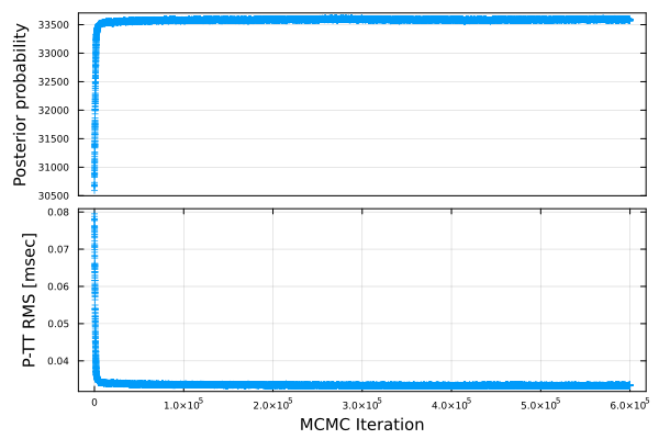
Parameter variation through the MCMC iteration
When you'd like to check how the unknown parameters change through the MCMC iteration, you can draw by plot_mcmcparam_gradv(NA;fn,fno,show,nshuffle).
NA: Sampling interval of the MCMC prcessing (
NA=5by default), which must be same withNAinstatic_array_mcmcgradvfn: the input file name (
fn="sample.out"by default)fno: Output figure name (
fno="mcmc_param.pdf"by default)show: if
show=true, a figure is shown on REPL and is not saved as a file (show=falseby default)nshuffle: number of plots for each parameter (if all samples are plotted, the figure is crowded; thus,
nshuffleof samples are randomly picked; ifnshuffle=0, all samples are plotted;nshuffle=10000by default)
You can adjust the fontsizes or figuresize by the other arguments.
SeaGap.plot_mcmcparam_gradv(5,fno="mcmc_param.pdf")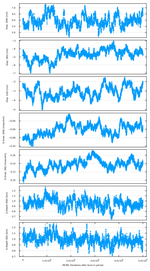
In this function, major six unknown parameters are shown. If you'd like to draw a figure for the other paramters, you can use plot_mcmcparam_each(param,NA;fn,fno,show,nshuffle). param is the parameter name written in "initial.inp".
SeaGap.plot_mcmcparam_each("S-NTD_10",5,fno="mcmc_param_S-NTD_10.png")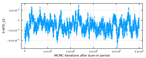
Correlation among the unknown parameters
When you'd like to simply check the trade-off relationship among the unknown parameters, you can draw a correlation map by plot_cormap_gradv(fn,fno0,fno,show,txt,all,as,pfs,plot_size).
fn: the input file name (
fn="sample.out"by default)fno0: Output text data file name (if
txt=true, correlation coefficients are save in this file;fno0="correlation.out")fno: Output figure name (
fno="cormap.pdf"by default)show: if
show=true, a figure is shown on REPL and is not saved as a file (show=falseby default)txt: Text data file output (
txt=falseby default)all: if
all=true, correlation coefficients are calculated for all parameters; ifall=false, correlation coefficients are calculated for major paramters (array displacements, shallow gradients, gradient depth)as: Fontsize of parameter names (
as=10by default)pfs: Fontsize of annotated correlation values (
pfs=8by default)plot_size: Figure size (
plot_size=()by default)
SeaGap.plot_cormap_gradv(fno="cormap.png")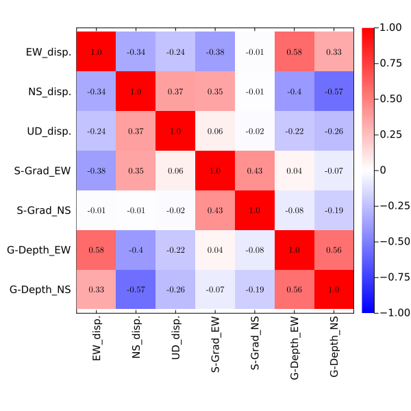
$ head -n 7 correlation.out | awk '{print $1,$2,$3,$4,$5,$6,$7}'
Name: EW_disp. NS_disp. UD_disp. S-Grad_EW S-Grad_NS G-Depth_EW
"EW_disp." 1.0 -0.3356124991185022 -0.23515279880381532 -0.3803514391901573 -0.011409026075565506 0.5828230015324758
"NS_disp." -0.3356124991185022 1.0 0.37266487444226404 0.3549474663596853 -0.006429289222325339 -0.39833730865946165
"UD_disp." -0.23515279880381532 0.37266487444226404 1.0 0.05928566131657452 -0.01530484319231686 -0.21752009435257144
"S-Grad_EW" -0.3803514391901573 0.3549474663596853 0.05928566131657452 1.0 0.42961339278338556 0.03768990735893968
"S-Grad_NS" -0.011409026075565506 -0.006429289222325339 -0.01530484319231686 0.42961339278338556 1.0 -0.07774179162939017
"G-Depth_EW" 0.5828230015324758 -0.39833730865946165 -0.21752009435257144 0.03768990735893968 -0.07774179162939017 1.0
Histogram for each unknown parameter
From the MCMC samples ("sample.out"), you can draw a histogram for each unknown parameter by plot_histogram_gradv(NPB1,NPB2,NPB3,NPB4;fn0,fn,fno,all,drawnls,nbins).
NPB1: Number of 3d B-spline bases for L-NTD
NPB2: Number of 3d B-spline bases for S-NTD
NPB3: Number of 3d B-spline bases for S-Grad
NPB4: Number of 3d B-spline bases for G-Depth
fn0: Inversion results by
static_array()("solve.out" by default), which is used when you'd like to plot thestatic_array()results on the histogramfn: Input file ("sample.out" by default)
fno: Output figure name (note that this file must be a PDF file: "histogram.pdf" by default)
all: if
all=true, histograms for all parameters are drawn; ifall=false, histograms for major six parameters (array displacements, shallow gradients, gradient depth) (all=falseby default)drawnls: if
drawnls=true, a normal distribution estimated bystatic_array()is drawn in a histogram (drawnls=falseby default); the normal distributions are shown for the array displacements and 3d B-spline NTDs. Note that you cannot use this option whenall=true.nbins: Number of histogram's intervals (
nbins=50by default)
SeaGap.plot_histogram(77,all=true,fno="histogram_all.pdf")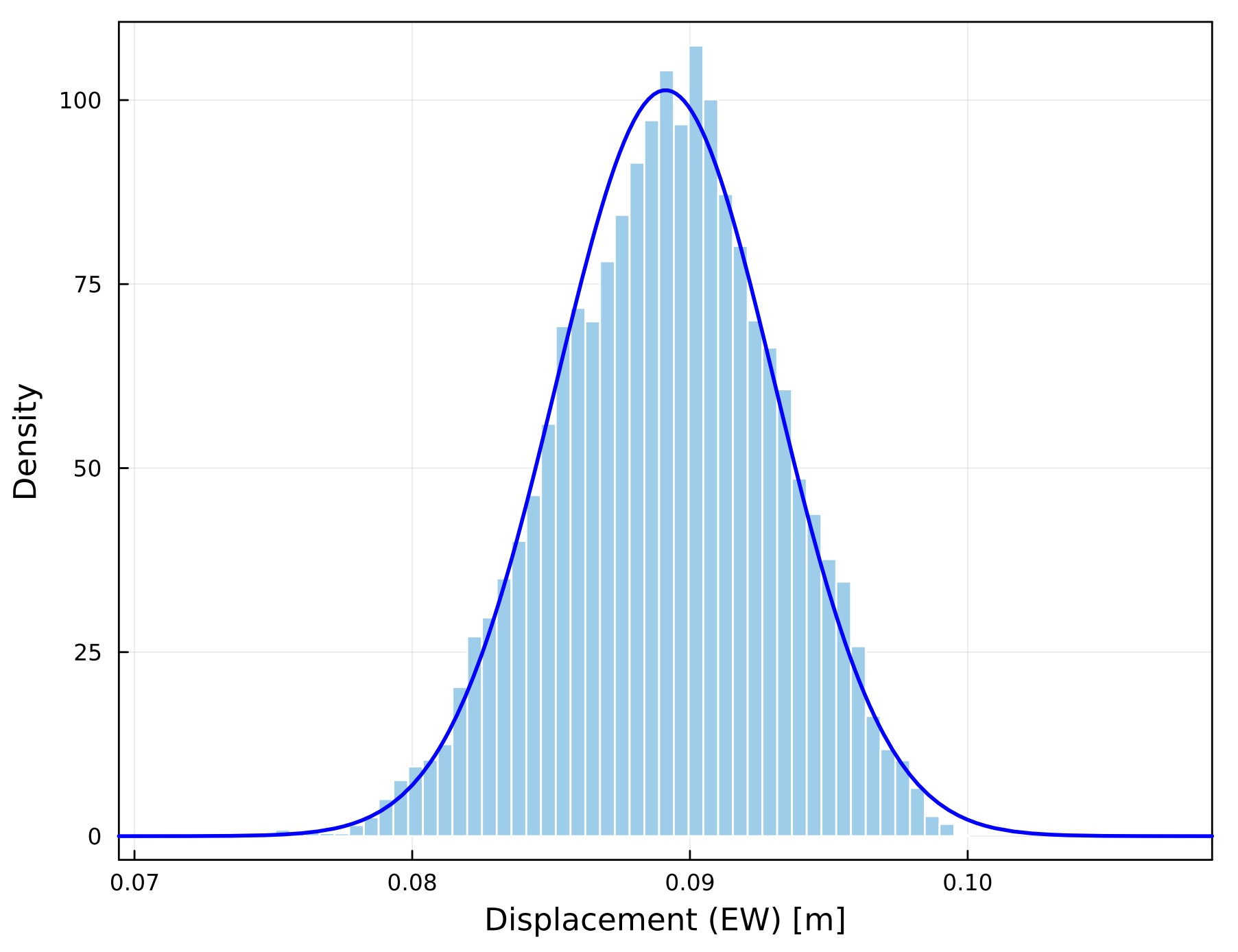
SeaGap.plot_histogram(77,all=true,fno="histogram_allv.pdf",drawnls=true)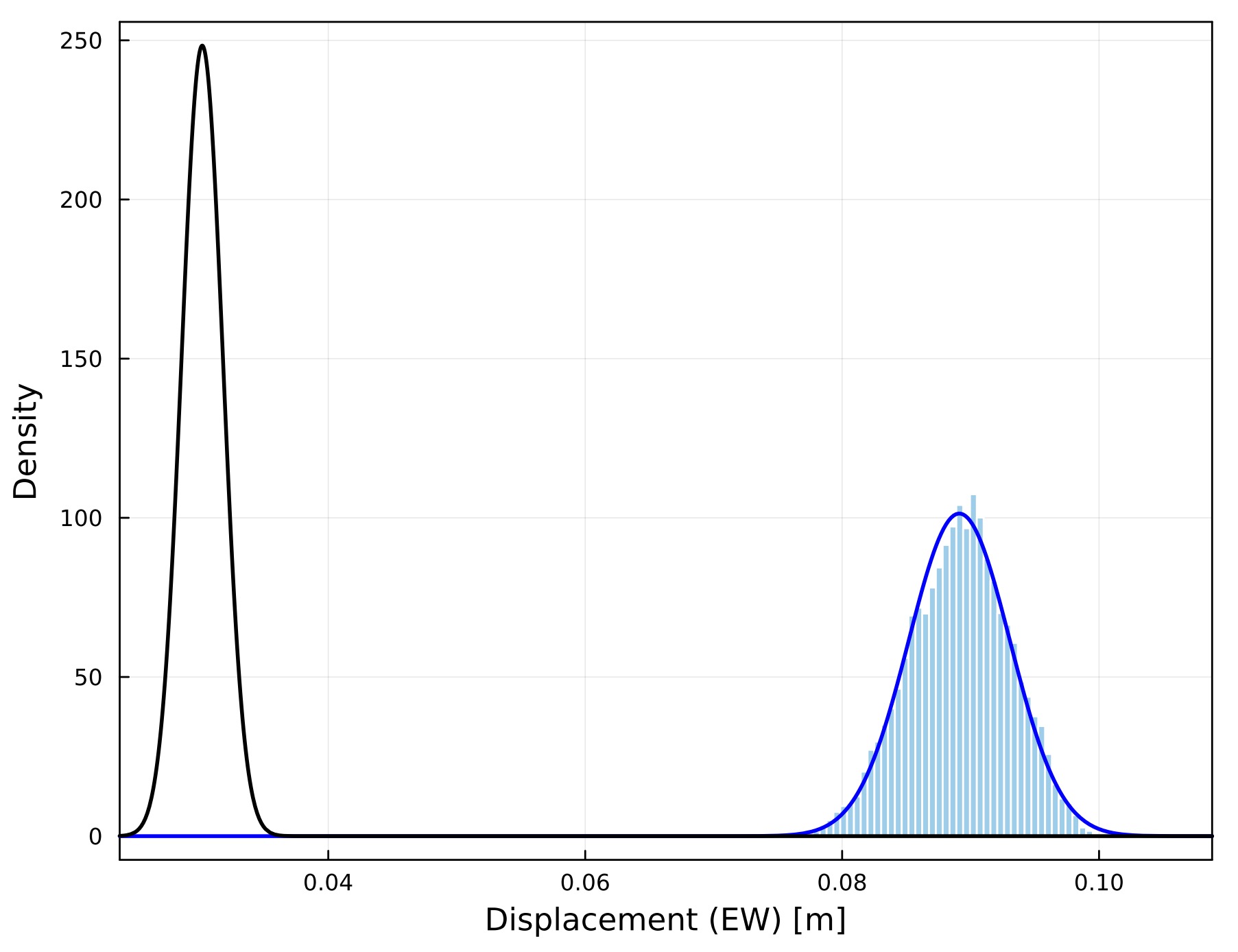
Histograms and heatmaps for multiple parameters
Using plot_histogram2d(fn,fno,show,nshufflei,nbins), you can draw a figure showing histograms, heatmaps, and scatter maps for major six parameters (array displacements, shallow gradients, gradient depth).
fn: Input file ("sample.out" by default)
fno: Output figure name
show: if
show=true, a figure is shown on REPL and is not saved as a file (show=falseby default)nshuffle: number of plots for each parameter (if all samples are plotted, the figure is crowded; thus,
nshuffleof samples are randomly picked; ifnshuffle=0, all samples are plotted;nshuffle=10000by default)nbins: Number of histogram's intervals (
nbins=50by default)
You can adjust fontsizes, margins of panels, and figure size by the other arguments.
SeaGap.plot_histogram2d(fno="histogram2d.pdf")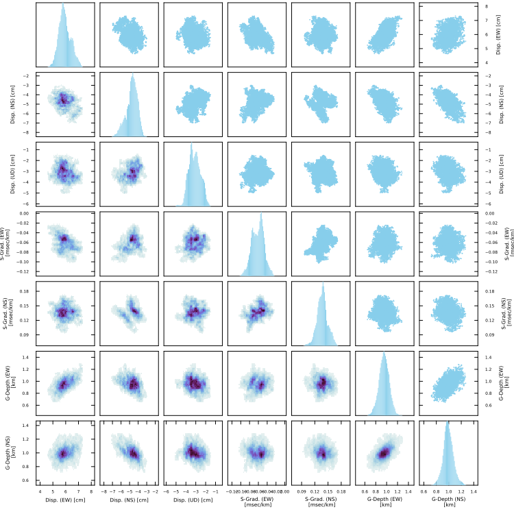
Diagonal panels show histograms for individual parameter. Upper triangle panels show scatter maps for corresponding two parameters. Lower triangle panels show heat maps for corresponding two parameters.
If you'd like to draw a heatmap for certain two parameters, you can make it by plot_histogram2d_each(param1,param2,fn,fno,show,nbins). param1 and param2 are the parameter names written in "initial.inp".
SeaGap.plot_histogram2d_each("UD_disp.","S-NTD_10",fno="histogram2d_UD_SNTD-10.png")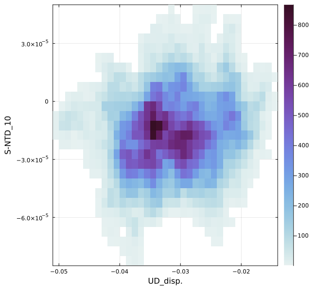
Spatial variation of travel-time residuals (shallow gardient)
plot_gradmap(xrange,yrange;autoscale,fn1,fn2,fno,show) draws a sea-surface platform track with color of the spatial variation due to the shallow gradients (the projected travel time residuals - L-NTD - S-NTD - D-Grad).
xrange: Range of EW component in meters when
autoscale=falseyrange: Range of NS component in meters when
autoscale=falseautoscale: If
autoscale=true, the plot range is automatically definedfn1: File name of the seafloor transponder positions ("pxp-ini.inp")
fn2: Travel-time residual file name ("residual_sdls.out")
fno: Output figure name ("gradmap.pdf" by default)
show: if
show=true, a figure is shown on REPL and is not saved as a file (show=falseby default)
SeaGap.plot_gradmap_gradv((-2500,2500),(-2500,2500),autoscale=false,fno="gradmap.png")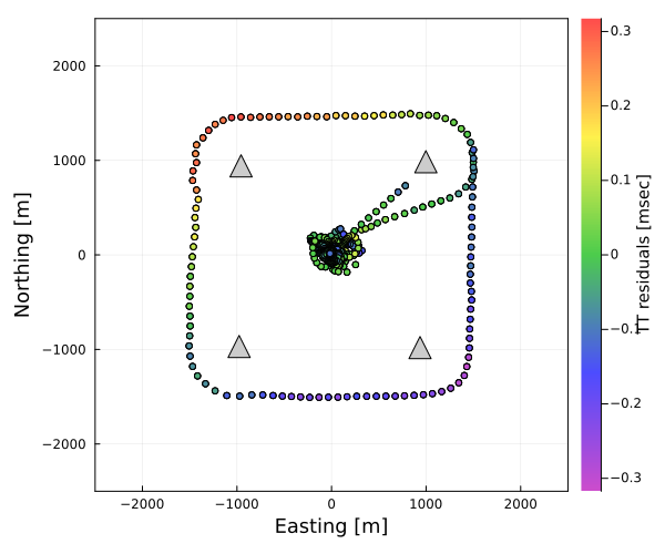
Temporal variation of the travel-time residuals
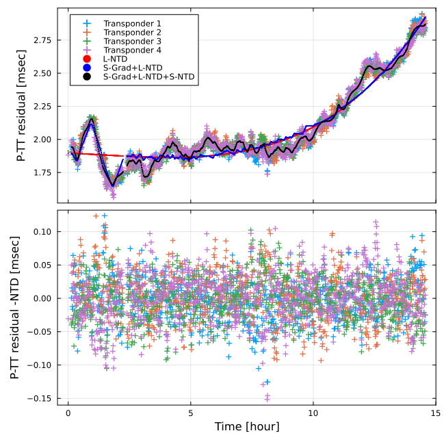
Time-series of the travel-time residuals are plotted by plot_ntd_gradv(ntdrange,resrange;autoscale,fn,fno,show).
ntdrange: Range of the upper two panels in msec when
autoscale=falseresrange: Range of the lowest panels in msec when
autoscale=falseautoscale: If
autoscale=true, the plot range is automatically definedfn: Travel-time residual file name ("residual_sdls.out")
fno: Output figure name ("ntdgrad.pdf" by default)
show: if
show=true, a figure is shown on REPL and is not saved as a file (show=falseby default)
SeaGap.plot_ntd_gradv()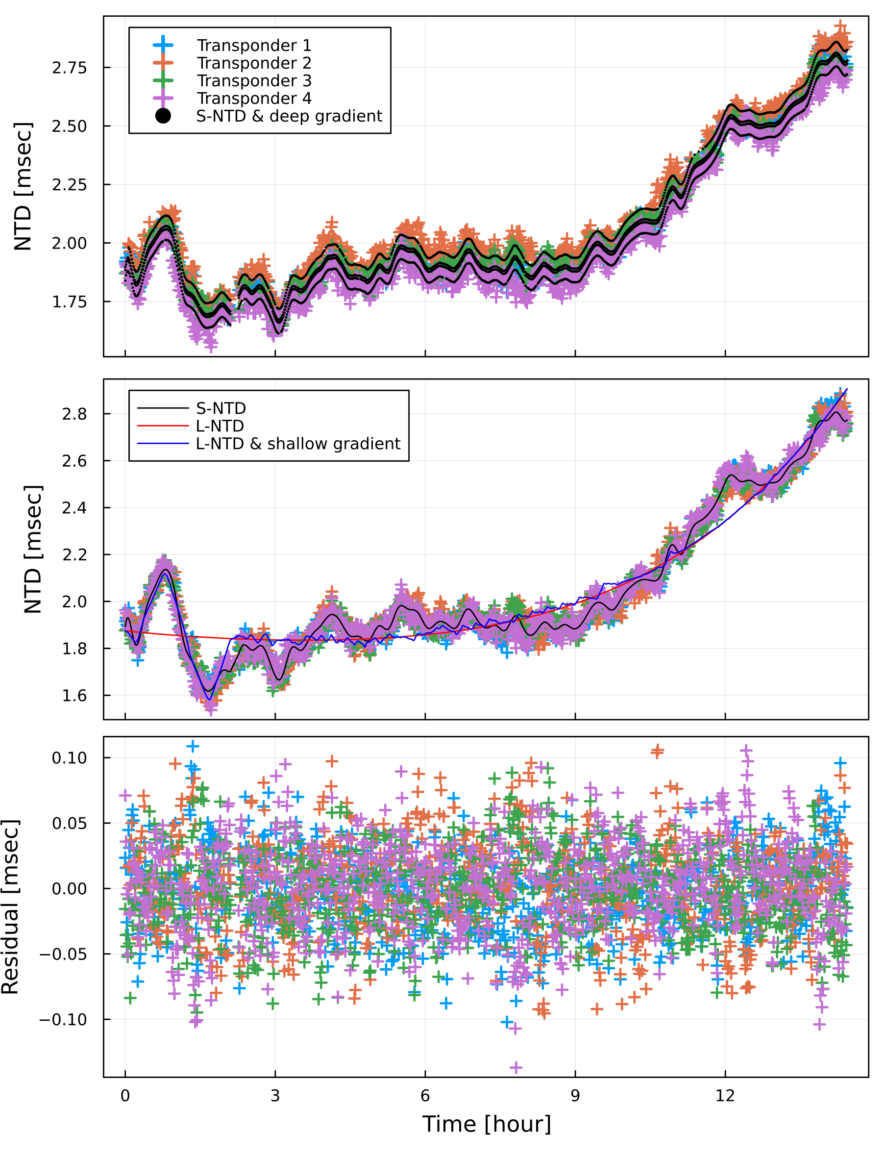
The upper panel shows the projected travel-time residuals by cross symbols. Moreover, black dots show combination of the 3d B-splined NTD and the deep gradient contribution.
The middle panel shows the projected travel-time residuals subtracting the deep gradient contribution by cross symbols. Moreover, the 3d B-splined NTD, the long-term NTD, and combination of the long-term NTD and the shallow gradients are shown by black, red, and blue curves, respecively.
The lower panel shows the final travel-time residuals.
CC BY-SA 4.0 Fumiaki Tomita. Last modified: July 03, 2024.
Website built with Franklin.jl and the Julia programming language.