Tutorials

Static array positioning

Basic static array positioning
Optimization of the total number of 3d B-spline bases
Optimization of the transducer-antenna offset
Static array positioning directly estimating deep gradients

In SeaGap, the static positioning function (static_array) based on Tomita & Kido (2022) is provided. A static array position and coefficients for the 3d B-spline functions can be estimated by Gauss-Newton method. Moreover, to optimize the number of the 3d B-spline bases, SeaGap has a function to calculate AIC and BIC values for various number of the 3d B-spline bases (static_array_AICBIC). As a derived function from static_array, a function static_array_TR additionally estimates an offset between a transducer and a GNSS antenna.

Basic static array positioning

To perform static_array, you have to prepare four input files denoted in Dataformat: "tr-ant.inp". "pxp-ini.inp", "ss_prof.inp", and "obsdata.inp". Outliers in "obsdata.inp" should be removed in advance; SeaGap includes a simple outlier removal function.

The basic static array positioning static_array() can be performed as following:

lat=36.15753; TR_DEPTH=[4.0]; NPB=100
SeaGap.static_array(lat,TR_DEPTH,NPB)

To perform static_array(), you have to provide the site latitude and the rough depth of transducer from the sea-surface at the first and second arguments, respectively, as indicated in the previous pages (Forward calculation and Kinematic array positioning). Moreover, you also have to provide number of the 3d B-spline bases at the third argument. Here, we provided 100 bases for instance.

The input files are fn1, fn2, fn3, and fn4; they correspond to "tr-ant.inp". "pxp-ini.inp", "ss_prof.inp", and "obsdata.inp" by default. If you use the default file names, you need not to denote as arguments.

Then, after performing, you obtained a log file as fno0 (fno0="log.txt" by default), a solution file fno1 (fno1="solve.out"), a position file fno2 (fno2="position.out"), a NTD file fno3 (fno3="residual.out"), a B-spline function file fno4 (fno4="bspline.out"), and a AIC/BIC file fno5 (fno5="AICBIC.out").

fno1 shows the estimated values for the all unknown paramters (Column 1) and their estimated errors (Column 2). First three paramters are the array displacement in meter (Line 1: EW, 2: NS, 3: UD), and the followings are the coeffiecnts for the 3d B-spline bases.

$ head solve.out

0.025569840487938453   0.0016129310076125585
 -0.015875407745997182   0.001613186827589505
 -0.03376358011884562    0.0059052501621037635
  0.0028292312669924583  0.0006405078846468068
  0.0015882479862308909  0.00014936310584887032
  0.002053655747197      3.207183443888804e-5
  0.0018425944267670055  1.803903131510534e-5
  0.001847072424717548   1.465345165678352e-5
  0.002055841628452572   1.4064308009718126e-5
  0.0020628606036604915  1.395626180639233e-5

fno2 shows general positioning results (1: Average observational time (cumulative seconds from the reference time), 2-4: the estimated array displacements in EW, NS, and UD, 5-7: 1 $\sigma$ estimation errors in EW, NS, and UD).

$ cat position.out

5.00690645363141e8  0.025569840487938453  -0.015875407745997182  -0.03376358011884562  0.0016129310076125585  0.001613186827589505  0.0059052501621037635

fno3 shows the modeled results for NTD:

1: the observational time (cumulative seconds from the reference time)
2: Site number
3: Normalized travel-time residuals $\frac{1}{M\left(\xi_{n,k}\right)}T^{\rm obs}_{n,k}-\frac{1}{M\left(\xi_{n,k}\right)}T^{\rm cal}\left({\bf u}(t_n, {\bf b}_0),{\bf p}_k+\delta{\bf p},v_0\right)$
4: Modeled NTD ( $\sum_{j=1}^{J}c_j\Phi_j(t_n)$ )
5: Residuals between the columns 3 and 4

$ head residual.out

5.00664410095011e8    4.0  0.0018449755930877668  0.0018705469372877442  -2.5571344199977388e-5
 5.00664440093926e8    4.0  0.0018824868863634263  0.001852118115376272    3.0368770987154346e-5
 5.00664920015051e8    1.0  0.0019435072397675811  0.0019334436223810048   1.0063617386576367e-5
 5.0066492022755253e8  3.0  0.0019030245459480146  0.0019336373718999381  -3.0612825951923566e-5
 5.0066492010527e8     4.0  0.001992831510936241   0.001933613539532501    5.921797140373986e-5
 5.0066498000643504e8  1.0  0.001958258457199361   0.0019472420380419      1.1016419157460888e-5
 5.00664980241396e8    3.0  0.0019055709885397217  0.0019474118171821846  -4.1840828642462826e-5
 5.00664980102315e8    4.0  0.001980233643143951   0.0019473994136280399   3.283422951591108e-5
 5.00665039994504e8    1.0  0.0019288464605689234  0.001953450397784169   -2.4603937215245727e-5
 5.006650402641685e8   3.0  0.0019090429001348119  0.001953594042111864   -4.4551141977051956e-5

fno4 shows the modeled results of B-spline function:

1: number of the 3d B-spline bases
2: usable ID (if the corresponding basis is not used in the modeling, ID = 0)
3: the observational time (cumulative seconds from the reference time)
4: the estimated coefficents of the 3d B-spline bases

$ head bspline.out

1.0    1.0  5.0066386599961245e8  0.0028292312669924583
   2.0    2.0  5.00664407e8          0.0015882479862308909
   3.0    3.0  5.0066494800038755e8  0.002053655747197
   4.0    4.0  5.006654890007751e8   0.0018425944267670055
   5.0    5.0  5.0066603000116265e8  0.001847072424717548
   6.0    6.0  5.006665710015502e8   0.002055841628452572
   7.0    7.0  5.0066711200193775e8  0.0020628606036604915
   8.0    8.0  5.006676530023253e8   0.0021528459136856935
   9.0    9.0  5.0066819400271285e8  0.0021431008849452315
  10.0   10.0  5.006687350031004e8   0.0019811296227287053

fno5 shows AIC and BIC values:

1: total number of the 3d B-spline bases
2: AIC
3: BIC

$ cat AICBIC.out

100 -68800.74652164285 -68170.78632318709

You can change analysis conditions by the keyword arguments:

eps: Convergence criteria [m], the default is 1.e-4 (each inversion is conve

rged when RMS of difference between the previous and the new solutions of the ho rizontal array displacements < eps)

ITMAX: Maximum number of interations, the default is 50
delta_pos: Infinitesimal amount of the array positions to calculate the Jacobian matrix, the default is 1.e-4 [m]

For example,

SeaGap.static_array(lat,TR_DEPTH,NPB,delta_pos=1.e-5)

The time-series of NTD (temporal sound speed fluctuation) is summarized in fno3="residual.out", and it can be visualized by plot_ntd(ntdrange,resrange; autoscale,fn,fno,show)

If autoscale=true (default), the plot range is automatically determined. If autoscale=false, the plot range of y-componet is fixed by ntdrange and resrange. The range of x-compoent (Time) is automatically determined in the both cases.
fn is the input file name: "residual.out" by default.
If show=false, the figure is saved as fno (fno is name of the output figure: "ntd.pdf" by default). If show=true in REPL, a figure is temporally shown.

SeaGap.plot_ntd(fno="ntd.pdf")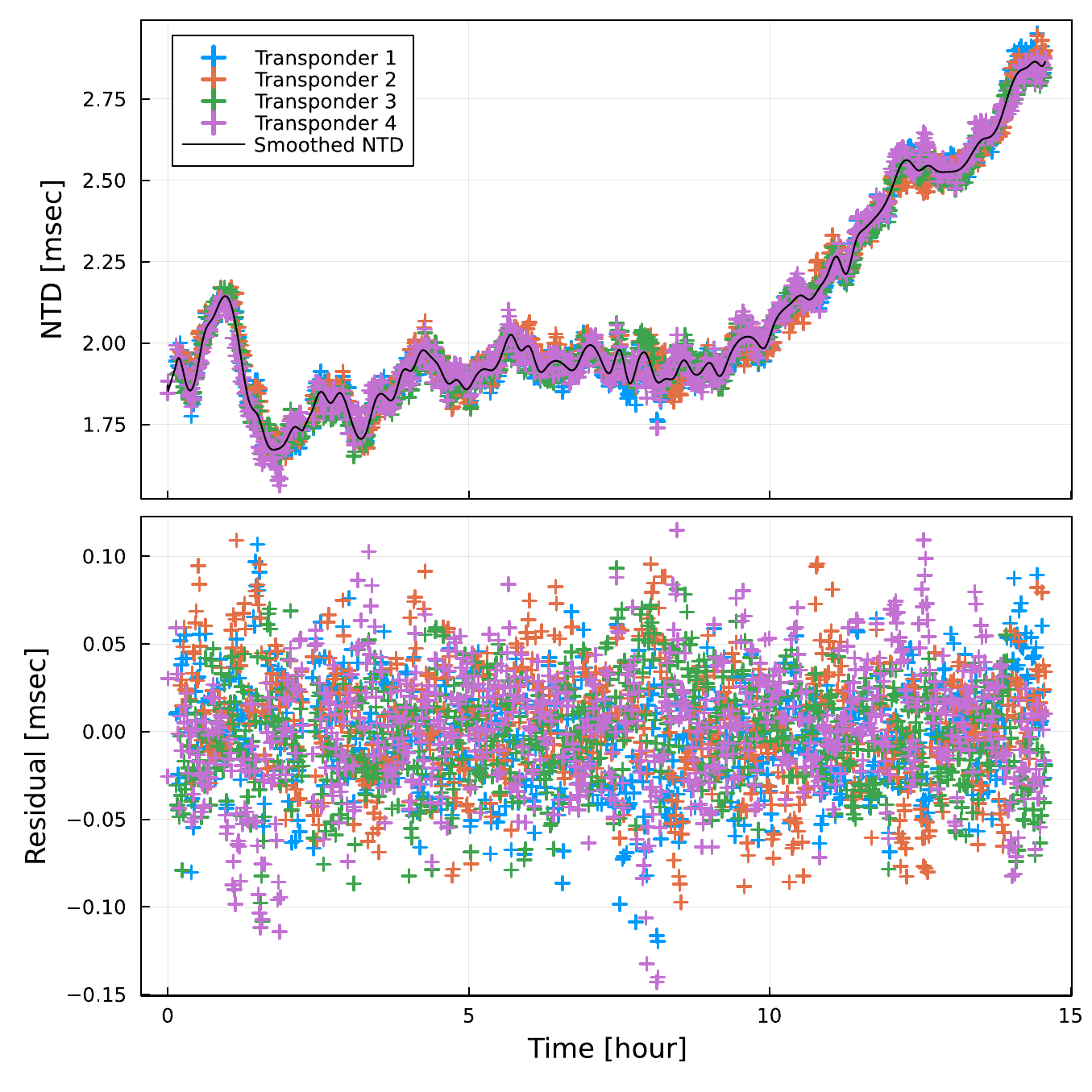

Top panel

The colored plots show the normalized travel-time residuals $\frac{1}{M\left(\xi_{n,k}\right)}T^{\rm obs}_{n,k}-\frac{1}{M\left(\xi_{n,k}\right)}T^{\rm cal}\left({\bf u}(t_n, {\bf b}_0),{\bf p}_k+\delta{\bf p},v_0\right)$ . Note that $T^{\rm cal}$ is calculated from the optimized seafloor transponder positions. The black curve shows the optimized NTD fluctuation modeled by the 3d B-spline functions.

Bottom panel

The final travel-time residuals for each seafloor transponder are shown, which correspond to the colored plots subtracting the black curve in the top panel.

Optimization of the total number of 3d B-spline bases

In SeaGap, the bases of the 3d B-spline function are deployed with temporally constant intervals, and the number of them can be optionally provided. The number of the bases of the 3d B-spline function directly affects temporal smoothness of the modeled NTD fluctuation so that it should be optimized depending on the observational data.

static_array_AICBIC(r1,r2,r3,lat,TR_DEPTH; fno,delete) is a function to calculate AIC and BIC for various number of 3d B-spline bases. r1, r2, and r3 are all integers expressing the search range: minimum, maximum, and interval number, respectively.

For example,

SeaGap.static_array_AICBIC(30,150,5,lat,TR_DEPTH)

As a result, you obtain fno (the output file: "AICBIC_search.out" by default) showing (1: Total number of 3d B-spline bases, 2: AIC, 3: BIC, 4: RMS [sec]).

$ head AICBIC_search.out

30 -67594.35388945481 -67392.5219812117 4.089131458631897e-5
35 -67878.3261641564 -67645.91366375524 3.913491415663497e-5
40 -68061.21208324382 -67798.21899068462 3.8023670469485674e-5
45 -68075.53192749251 -67781.95824277526 3.788581914518492e-5
50 -68115.25130917276 -67791.09703229746 3.7605549809629455e-5
55 -68212.0453944058 -67857.31052537245 3.701053875721755e-5
60 -68351.01091684843 -67965.69545565704 3.619625865943626e-5
65 -68448.25769269654 -68032.3616393471 3.562113772432889e-5
70 -68540.5609666159 -68094.08432110841 3.508104482907046e-5
75 -68664.8326454064 -68187.77540774086 3.4384587648691415e-5

You can check the results by plot_AICBIC(;type,fn,fno,show). You set type as "AIC" or "BIC". fn is the input file ("AICBIC_search.out" by default) for plot. If show=false, the plot is saved as fno (fno is the figure name; "AICBIC_search.pdf" by default). If show=true, the plot is temporally shown on REPL.

SeaGap.plot_AICBIC(type="BIC",show=true)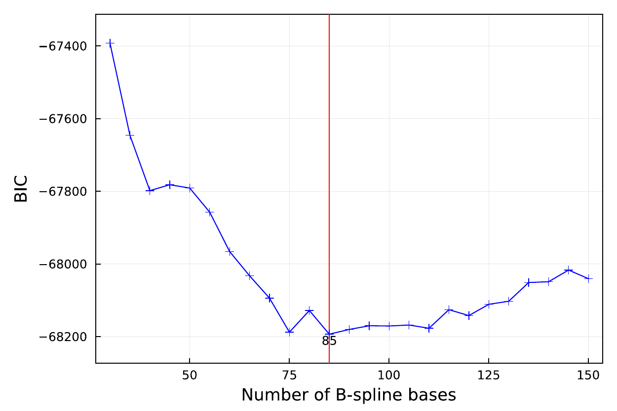

The number of 3d B-spline bases with the minimum criterion is shown by a red vertical line.

If you'd like to check in detail, you can additionally perform static_array_AICBIC():

SeaGap.static_array_AICBIC(61,99,1,lat,TR_DEPTH)

The AIC and BIC values are additionally written in fno (the output file: "AICBIC_search.out" by default). If you'd like to save the results in a new file, you add delete=true.

SeaGap.plot_AICBIC(type="BIC",fno="BIC_search.png")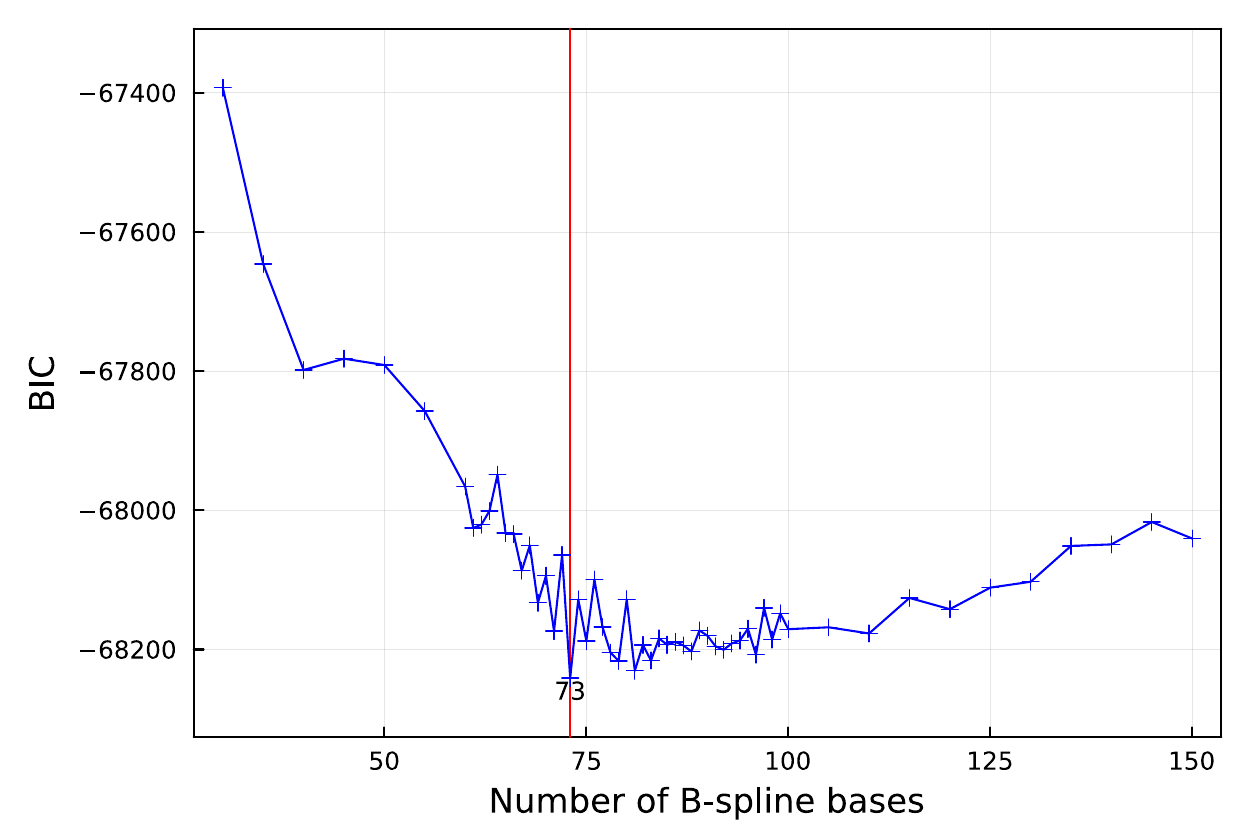

Optimization of the transducer-antenna offset

pos_array_TR() performs the static array positioning with optimization of an offset between a transducer and a GNSS antenna. The initial values of the offset are shown in fn1="tr-ant.inp".

lat=36.15753; TR_DEPTH=[4.0]; NPB=73; key=1
SeaGap.static_array_TR(key,lat,TR_DEPTH,NPB)

This function optimizes the offset for the key identifying number of the sea surface platforms. The other arguments and the input/output files of static_array_TR() are same with those of static_array() except fno1, fno5, and delta_offset. fno1 shows the estimated values for the all unknown paramters (Column 1) and their estimated errors (Column 2) as same with static_array(), and its file name is "solve.out" by default. However, the lines 4-6 in fno1 shows the solutions and the errors for the modification values of the offset from the initial file (fn1="tr-ant.inp").

fno5 in static_array_TR() shows three components of the estimated offset values and their estimation errors (1-3: Offset in X, Y, Z, 4-6: Error in X, Y, Z). The default name of fno5 is "tr-ant.out"

$ cat tr-ant.out

# TR_offset: dx, dy, dz, sigmax, sigmay, sigmaz
0.3616906760091636 17.724424295279814 -11.384094674905342 0.002220912736952465 0.002122249262876749 0.021302808617137618

Note that the estimated offset (especially in Z component) and the error are strongly influenced by delta_offset which is a infinitesimal value to calculate the Jacobian matrix.

You can make a figure on NTD fluctuation using plot_ntd().

Static array positioning directly estimating deep gradients

static_array_grad() is a function to estimate the array position, NTD, and the deep gradient following the observation equation (0) shown in Methodolgy.

lat=36.15753; TR_DEPTH=[4.0]; NPB=73
SeaGap.static_array_grad(lat,TR_DEPTH,NPB)

The input and output files are same with static_array() except fno1 (solve.out). fno1 shows the estimated values for the all unknown paramters (Column 1) and their estimated errors (Column 2). First three paramters are the array displacement in meter (Line 1: EW, 2: NS, 3: UD), following two parameters are the deep gradients (EW and NS components), and the followings are the coeffients for the 3d B-spline bases.