Line fitting for time-series

After positioning multiple campaign, you would perform time-series analysis for assessing crustal deformation. The general positioning results are shown in "position.out" by static_array(), static_array_mcmcgrad(), static_array_mcmcgradc(). You can obtain time-series of the array displacements by merging the "position.out" for multiple campaigns.

But, you should correct a stable plate motion to consider long-term crustal deformation (e.g., inter-/post-seismic deformation). After the correction, it is generally performed to calculate a displacement rate.

SeaGap provides functions to arrange (including a function to elimiate a constant velocity) the merged "position.out" and to calculate an array displcament rate.

First, let's prepare the merged "position.out" as "position_merge.out".

406823232 -0.096889228 0.139634124 -0.334569674 0.01040281 0.01023568 0.31545639
427997740 -0.023633200 0.053856194 0.080438784 0.00262383 0.00164626 0.00407914
446630293 -0.086322921 0.016209885 0.078556148 0.00487531 0.00100381 0.00372393
478175535 0.047437107 -0.018050471 0.073543488 0.00103975 0.00104308 0.00287912
500691126 0.045814082 -0.040725985 -0.028688630 0.00258226 0.00301437 0.00371223
515402741 0.035828374 -0.088293375 0.064555567 0.00352865 0.00311975 0.00899014
561563695 0.060865355 -0.045373625 0.101002939 0.01289510 0.01039353 0.02149323

Then, the merged position file should be arranged, and a constant velocity (a stable plate motion) should be eliminated. These can be performed by convert_displacement(vx,vy,vz;redu,sredu_hor,sredu_ver,fno,fn,t0).

• vx, vy, vz: constant velocities which are eliminated from the time-series (Unit: cm/yr)

• redu: if redu=true, the large estimation errors are identified as unusable (estimation errors in EW and NS components > sredu_hor; those in UD component > sredu_ver); if redu=false, all are identified as usable

• sredu_hor: Estimation error limit to be usable for horizontal components (sredu_hor=30.0 [cm] by default)

• sredu_ver: Estimation error limit to be usable for vertical component (sredu_ver=30.0 [cm] by default)

• fno: Arranged time-series file ("converted_position.out" by defalult)

• fn: Input time-series file ("position_merge.out" by defalult)

• t0: Reference time ("2000-01-01T12:00:00" by default; refer Date & Time processing [e.g., sec2year()])

SeaGap.convert_displacement(1.79,-1.79,0.0,sredu_hor=30.0,sredu_ver=30.0,fno="converted_position.out")

# Year DispX DispY DispZ SigmaX SigmaY SigmaZ UsableX UsableY UsableZ (detrend 1.79 -1.79 0.0)
2012.89344 -9.689 13.963 -33.457 1.040 1.024 31.546 1 1 0
2013.56438 -3.564 6.587 8.044 0.262 0.165 0.408 1 1 1
2014.15342 -10.888 3.876 7.856 0.488 0.100 0.372 1 1 1
2015.15342 0.698 2.240 7.354 0.104 0.104 0.288 1 1 1
2015.86849 -0.744 1.253 -2.869 0.258 0.301 0.371 1 1 1
2016.33333 -2.575 -2.672 6.456 0.353 0.312 0.899 1 1 1
2017.79726 -2.691 4.240 10.100 1.290 1.039 2.149 1 1 1

As shown above, the cumulative time [sec] is converted into AD [year] (Column 1); units of the array displacements and thier estimation errors [m] are converted into [cm] (Columns 2-7); constant velocities (vx,vy,vz) are eliminated from the array displacements (Columns 2-4); Columns 8-10 indicate usable/unusable (1/0) for each component. It doen't matter to produce this file your own way.

Using "converted_position.out", plot_displacement(ts,te,EW_range,NS_range,UD_range;autoscale,pscale,sigma,cal,weight,predict,fno1,fno2,fno3,fn,show) calculates an array displacement rate for each component and make a figure.

• ts: Start time of the figure (Time at the left edge of the figure) [yr]

• te: End time of the figure (Time at the right edge of the figure) [yr]

• EW_range, NS_range, UD_range: If autoscale=false, the range of Y-axis is set to be those ranges

• autoscale: if autoscale=true (default), the range of Y-axis is automatically determined depending on the usable array displacements

• pscale: if you set smaller value, the autoscale Y-axis range is wider (pscale=0.5 by default)

• sigma: Errorbar scaling (Since standard deviation of an array displacement tends to be small, the plotting errorbar is multiplied by sigma: sigma=10 by default)

• cal: if cal=true, a regression line is calculated for each component, is shown in the figure, and the regression results are written in fno2 as a text file

• weight: if weight=true, the regression line is calculated considering the weight; the weight is provided as an inverse square of the observation error (weight=true by default)

• predict: if predict=true, the predicted values from the regression line are written in "fno3-EW.txt", "fno3-NS.txt", and "fno3-UD.txt"

• fno1: Output figure name

• fno2: Name of an output text file showing array displacement rates

• fno3: Indicator name of output text files showing the predicted values from the regression lines

• fn: Input file name ("converted_position.out")

• show: If show=false, the figure is saved as fno (fno is name of the output figure). If show=true in REPL, a figure is temporally shown.

SeaGap.plot_displacement(2012,2018.5,fno1="displacement.png")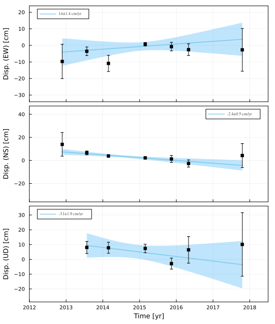

SeaGap.plot_displacement(2012,2018.5,(-25,15),(-10,30),(-40,40),fno1="displacement_wo.png",autoscale=false,cal=false)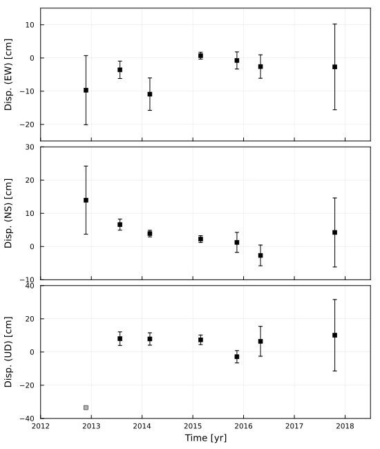

The thick blue line shows a regression line for each component, and the shaded portion shows a 95% confidence interval. Glay and black squares are the unusable and usable array displacements, respectively.

The regression results are given as following:

# (Vx,Vy,Vz,Sx,Sy,Sz,RMSx,RMSy,RMSz,CorXY) in cm Linear model
1.5742551020532471 -2.3877121258416882 -3.0700998568383113 1.3995537945799512 0.5303522727297605 1.8953362710629817 11.569073350333905 6.4632288773323445 9.787610128634833 -0.3291858072408599 7 7 6

# Year Disp. Pred. Residual Sigma
 2012.89344   -9.689  -4.025397254303815   -5.663602745696185   1.04
 2013.56438   -3.564  -2.969166536132252   -0.5948334638677482  0.262
 2014.15342  -10.888  -2.0418673108187     -8.8461326891813     0.488
 2015.15342    0.698  -0.4676122087654528   1.1656122087654528  0.104
 2015.86849   -0.744   0.6580903870597136  -1.4020903870597134  0.258
 2016.33333   -2.575   1.389867128697936   -3.9648671286979362  0.353
 2017.79726   -2.691   3.6944664002469327  -6.385466400246933   1.29